SAP Insiders
Articles/Finance and Controlling/Essential Costing Formulas in SAP S/4HANA — EOQ, Labour Cost, Overheads, and Cost Sheet
Finance and Controlling

Essential Costing Formulas in SAP S/4HANA — EOQ, Labour Cost, Overheads, and Cost Sheet

Every CA Inter costing formula has a direct SAP equivalent. This reference guide maps EOQ, Reorder Level, Labour Hour Rate, Machine Hour Rate, and the complete Cost Sheet waterfall to their SAP S/4HANA transaction codes.

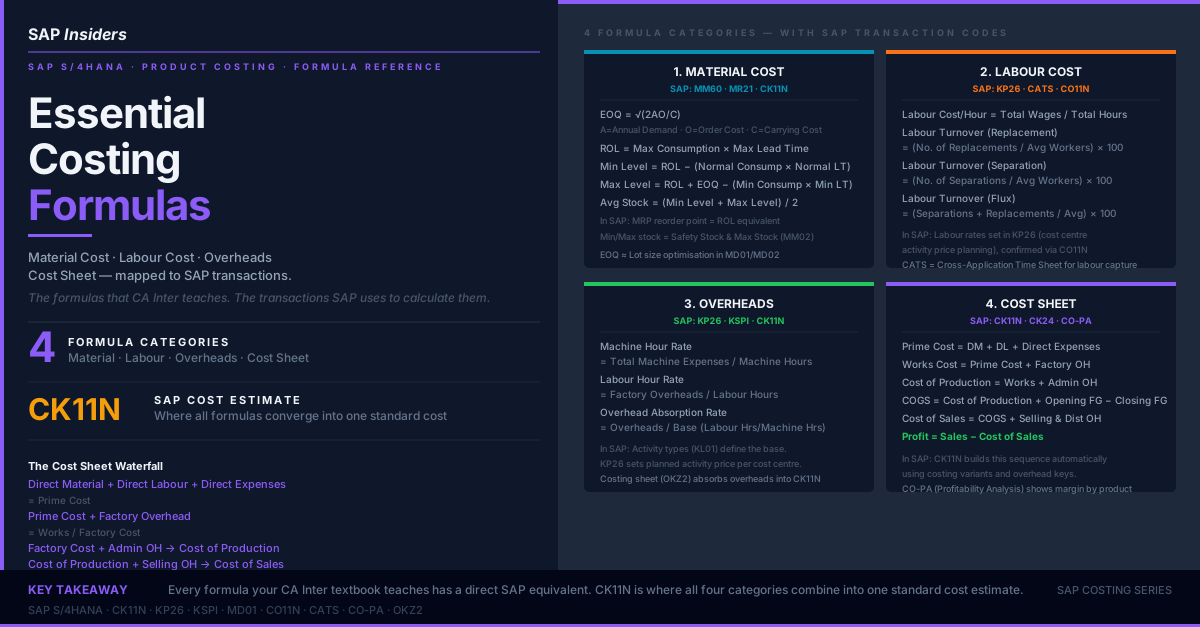
Enterprise dark infographic — Essential Costing Formulas in SAP S/4HANA covering Material Cost EOQ and reorder levels, Labour Cost, Overheads, and Cost Sheet waterfall mapped to SAP transactions

Glossary

EOQ (Economic Order Quantity) — the optimal order size that minimises total inventory costs (ordering cost + carrying cost). Formula: √(2AO/C).

Reorder Level (ROL) — the stock level that triggers a replenishment order. Formula: Maximum Consumption × Maximum Lead Time.

Activity Type — in SAP CO, a unit of capacity output from a cost centre. Examples: Machine Hours, Labour Hours, kWh. Used to absorb overhead into products.

Overhead Absorption Rate — the rate at which indirect costs are charged to products. Calculated as: Total Overhead / Base (hours, units, or value).

Costing Sheet — SAP configuration object (OKZ2) that defines how overheads are absorbed into a cost estimate or production order using overhead keys and rates.

CK11N — SAP transaction to create a standard cost estimate. Combines BOM quantities, routing times, material prices, and overhead rates into a per-unit standard cost.

KP26 — SAP transaction for cost centre activity price planning. Sets the planned rate per unit of activity (e.g. ₹350 per machine hour).


The costing formulas taught in CA Inter and ICWA are not abstract theory. Each one has a direct operational equivalent in SAP S/4HANA — a configuration object, a transaction code, or a planning process. This guide maps each formula category to how SAP implements it.


Category 1 — Material Cost

EOQ — Economic Order Quantity

EOQ = √(2AO/C)

Where:
A = Annual Demand (units)
O = Ordering Cost per order (₹)
C = Carrying Cost per unit per year (₹)

Example: Vajra Precision Tools orders steel billets 1,200 times a year. Each order costs ₹800 in administrative and transport costs. Annual carrying cost per tonne is ₹1,200.

EOQ = √(2 × 1,200 × 800 / 1,200) = √1,600 = 40 tonnes per order

In SAP: EOQ appears as lot sizing in the material master (MM02, MRP 1 view). SAP's lot sizing procedures include Fixed Lot Size (FX), Periodic Lot Size (monthly/weekly), and the Economic Order Quantity calculation (WB — optimum lot size). The MRP run (MD01/MD02) uses the lot size to generate planned orders or purchase requisitions.

Reorder Level (ROL)

ROL = Maximum Consumption × Maximum Lead Time

Minimum Level = ROL − (Normal Consumption × Normal Lead Time)

Maximum Level = ROL + EOQ − (Minimum Consumption × Minimum Lead Time)

Average Stock Level = (Minimum Level + Maximum Level) / 2

Example:

  • Max consumption: 50 tonnes/week
  • Max lead time: 4 weeks
  • Normal consumption: 35 tonnes/week, Normal lead time: 3 weeks
ROL = 50 × 4 = 200 tonnes
Min Level = 200 − (35 × 3) = 200 − 105 = 95 tonnes
Max Level = 200 + 40 − (20 × 2) = 240 − 40 = 200 tonnes
Average Stock = (95 + 200) / 2 = 147.5 tonnes

In SAP: Reorder level maps to the reorder point in MM02 (MRP 1 view). Min Level maps to Safety Stock (MRP 2 view). Max Level maps to Maximum Stock Level (MRP 2 view). When stock falls below the reorder point, MRP automatically generates a purchase requisition.

FormulaSAP FieldTransaction
EOQLot Size / Fixed LotMM02, MRP 1
ROL (Reorder Level)Reorder PointMM02, MRP 1
Minimum LevelSafety StockMM02, MRP 2
Maximum LevelMaximum Stock LevelMM02, MRP 2

Q: Vajra's steel billet has a reorder point of 200 tonnes in SAP. Current stock is 210 tonnes. A production order needs 80 tonnes. Will MRP trigger a purchase requisition after the next planning run?

A: Yes. After the goods issue for the production order, stock will drop to 130 tonnes — below the reorder point of 200. The next MRP run (MD01/MD02) will generate a purchase requisition for the EOQ quantity.


Category 2 — Labour Cost

Labour Cost per Hour

Labour Cost per Hour = Total Wages / Total Hours Worked

Example: A machining cost centre at Vajra has 12 operators each earning ₹25,000/month including all statutory contributions. Total hours available per month: 12 × 160 = 1,920 hours.

Labour Cost per Hour = (12 × ₹25,000) / 1,920 = ₹3,00,000 / 1,920 = ₹156.25/hour

In SAP: This rate is set in KP26 (cost centre activity price planning). The controller enters the planned total cost for the labour activity type and the planned quantity (hours). SAP calculates the planned rate per hour automatically.

Labour Turnover

Labour Turnover (Replacement Rate)
= (Number of Replacements / Average No. of Workers) × 100

Labour Turnover (Separation Rate)
= (Number of Separations / Average No. of Workers) × 100

Labour Turnover (Flux Rate)
= (Separations + Replacements / Average Workers) × 100

High labour turnover increases indirect labour costs: recruitment fees, training costs, onboarding time, and reduced productivity from new workers. These appear in the cost centre as indirect costs that get absorbed into products through the overhead rate.

In SAP: Labour turnover itself is not a standard SAP CO metric — it is captured in HR (Personnel Administration). However, its cost impact appears in the cost centre report (KSB1) as increased recruitment and training costs, which inflate the overhead rate when KP26 is planned.


Category 3 — Overheads

Machine Hour Rate

Machine Hour Rate = Total Machine-Related Expenses / Total Machine Hours

Machine-related expenses include: machine depreciation, maintenance, tooling, power consumption, and the portion of supervisor cost attributable to running the machines.

Example: The CNC machining centre at Vajra has ₹8,40,000 annual expenses. It operates 2,400 hours per year.

Machine Hour Rate = ₹8,40,000 / 2,400 = ₹350 per machine hour

In SAP: This is an activity type (transaction KL01) called "MACHINE_HR" assigned to the machining cost centre. The rate ₹350/machine hour is planned in KP26. When a production order is confirmed (CO11N), the system multiplies confirmed machine hours × ₹350 and debits the production order.

Labour Hour Rate

Labour Hour Rate = Total Factory Overheads / Total Labour Hours

This rate spreads indirect factory costs (indirect labour, factory rent, insurance, utilities) across products based on how many labour hours each product requires.

In SAP: If labour hours are used as the overhead base, a separate activity type "LABOUR_HR" is created (KL01) and planned in KP26. Alternatively, overheads can be absorbed using a costing sheet (OKZ2) as a percentage of direct labour cost — the simpler approach for facilities with many small products.

Overhead Absorption Rate

Overhead Absorption Rate = Total Overheads / Base

Base = Labour Hours OR Machine Hours OR Units Produced OR Direct Material Cost

Choosing the right base is critical:

BaseUse when
Machine HoursCapital-intensive processes where machine time drives overhead
Labour HoursLabour-intensive processes where people drive overhead
Units ProducedSingle-product facilities
Direct Material %Material-intensive products with minimal processing

In SAP: The overhead base is defined in the costing sheet (OKZ2 — Define Overhead). The overhead key specifies which overhead rates apply to which production orders. The costing run (CK11N) uses the costing sheet to absorb overhead into the standard cost estimate.

Q: Vajra has two production lines: a CNC machining line (capital-intensive, few workers) and an assembly line (labour-intensive, many workers). Should both lines use the same overhead absorption base?

A: No. The CNC line should use Machine Hour Rate (overhead driven by machine usage). The assembly line should use Labour Hour Rate (overhead driven by worker hours). In SAP, each cost centre can have its own activity type and rate — configure them separately in KP26.


Category 4 — Cost Sheet (The Complete Waterfall)

The cost sheet is the full build-up from raw input costs to selling price and profit. Every step has a SAP equivalent:

Direct Material                        ₹4,20,000
+ Direct Labour                        ₹  78,000
+ Direct Expenses                      ₹  12,000
                                      ─────────
= PRIME COST                          ₹5,10,000

+ Factory / Manufacturing Overhead     ₹1,02,000
                                      ─────────
= WORKS COST / FACTORY COST           ₹6,12,000

+ Administration Overhead              ₹  48,960
                                      ─────────
= COST OF PRODUCTION                  ₹6,60,960

+ Opening Finished Goods              ₹  50,000
− Closing Finished Goods              ₹ (30,000)
                                      ─────────
= COST OF GOODS SOLD (COGS)           ₹6,80,960

+ Selling & Distribution Overhead      ₹  34,048
                                      ─────────
= COST OF SALES                       ₹7,15,008

Net Sales                             ₹9,00,000
− Cost of Sales                       ₹7,15,008
                                      ─────────
= PROFIT                              ₹1,84,992   (Gross Margin: 20.6%)

How SAP builds this in CK11N

SAP's standard cost estimate (CK11N) builds the cost sheet automatically using:

Costing Variant (OKKN): Controls which prices are used for materials (standard price, moving average), which dates, and which costing version.

BOM (CS03): Supplies the material component list — quantities and material numbers for the direct material line.

Routing (CA03): Supplies the operations — activity types and quantities for direct labour and machine time.

Costing Sheet (OKZ2): Applies overhead percentages or rates to accumulate factory overhead, admin overhead, and selling overhead on top of the prime cost.

When CK11N runs, it reads all three structures and produces a layered cost estimate exactly matching the cost sheet waterfall above. The result is the standard cost per unit — which then drives COGS postings when goods are issued (MIGO).

CO-PA (Profitability Analysis): Takes the standard cost estimate and breaks it into margin components by customer, product, or region. This is where management can see gross margin, contribution margin, and net margin in one report (KE30).

Cost Sheet LineSAP Source
Direct MaterialBOM (CS03) × Material Standard Price
Direct LabourRouting (CA03) × Activity Rate (KP26)
Factory OverheadCosting Sheet (OKZ2) — overhead key
Admin OverheadCosting Sheet (OKZ2) — secondary overhead key
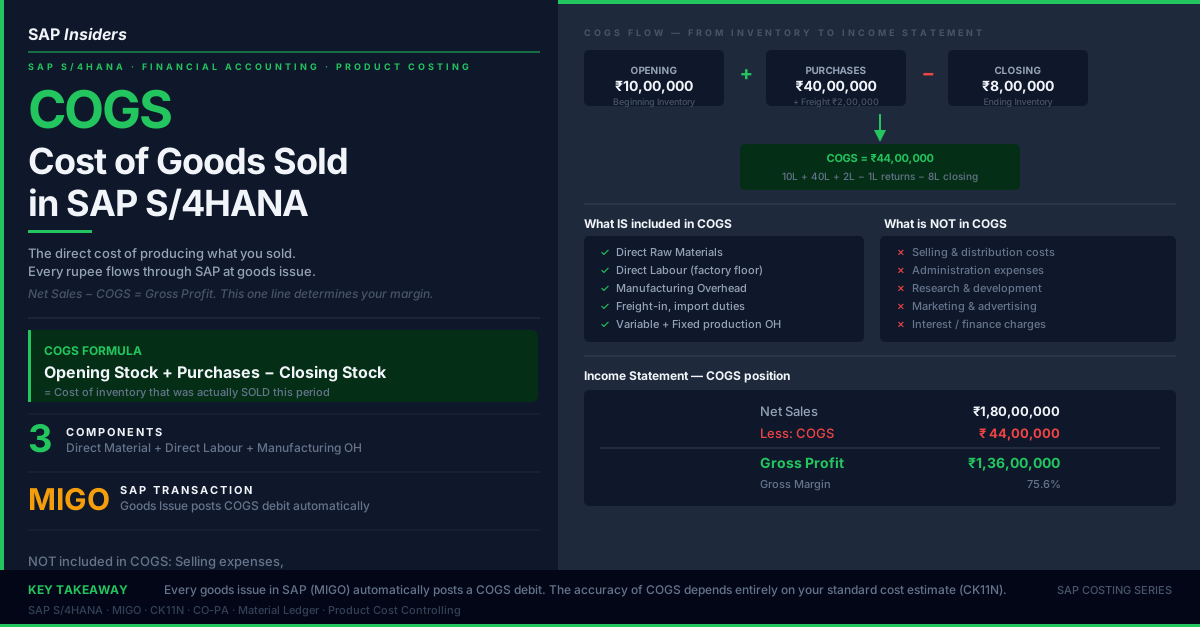
COGSCK11N standard cost × units sold (posted at MIGO)
Selling OverheadCO-PA value field or separate costing sheet row
ProfitCO-PA margin report (KE30)

Costing formulas reference cards — 4 quadrants showing Material Cost EOQ and ROL, Labour Cost rates and turnover, Overheads machine and labour hour rates, and Cost Sheet waterfall mapped to SAP transactions

The full SAP transaction map — costing formula to T-code

Formula CategoryFormulaSAP ImplementationT-Code
Material — EOQ√(2AO/C)Lot sizing in material masterMM02
Material — ROLMax Consump × Max LTReorder point in material masterMM02
Material — Safety StockMin LevelSafety stock fieldMM02
Labour — Rate/HourWages / HoursActivity price planningKP26
Labour — ConfirmationActual hours × rateProduction order confirmationCO11N
Overhead — Machine HRMachine Exp / Machine HrsMachine hour activity typeKL01, KP26
Overhead — Labour HRFactory OH / Labour HrsLabour hour activity typeKL01, KP26
Overhead — AbsorptionOH / BaseCosting sheet definitionOKZ2
Cost Sheet — Full buildDM + DL + OH waterfallStandard cost estimateCK11N
Cost Sheet — ReleaseMark and release standardActivate standard costCK24
COGS postingStandard cost × units soldGoods issueMIGO
Actual costActual costs vs standardMaterial Ledger actual costingCKMLCP
Margin by productSales − COGS − OHProfitability Analysis reportKE30

Putting it together — a costing month in SAP

Beginning of period (before first production):

  1. Review and update BOM if specifications changed (CS02)
  2. Update routings if machine speeds or labour grades changed (CA02)
  3. Run standard cost estimate (CK11N) and review cost components
  4. Mark and release the cost estimate (CK24) — this sets the standard price

During the period: 5. MRP runs daily/weekly — reorder points trigger purchase requisitions (MD01) 6. Production orders confirmed — CO11N records actual hours consumed 7. Goods issues posted — MIGO records actual material withdrawals 8. Sales deliveries posted — MIGO (601) triggers COGS at standard

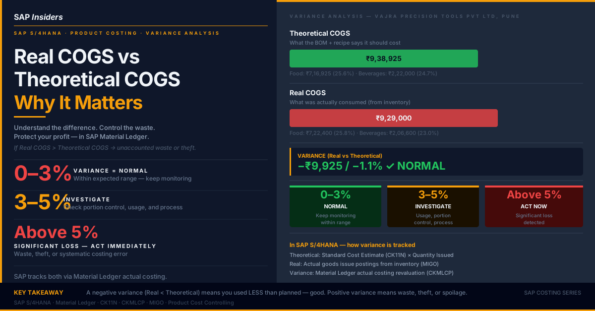
Period end: 9. Production orders settled (KO88) — variances calculated 10. Cost centre distribution/assessment (KSV5/KSU5) — indirect costs allocated 11. Material Ledger run (CKMLCP) — COGS revalued from standard to actual 12. CO-PA transfer (KE27) — margin data available in KE30 13. Compare Real COGS vs Theoretical COGS — identify variances above threshold

This sequence ensures that by the time the finance team closes the month, every rupee of cost has been traced from raw material through production to the income statement — with the variance between plan and actual clearly identified and explained.


This article is part of the SAP Insiders Costing Series. Previous articles: COGS — Cost of Goods Sold in SAP S/4HANA · Real COGS vs Theoretical COGS — Finding Hidden Waste.